
You’ll notice that the Function Arguments pane for the IF function has fields for Logical_test, Value_if_true, and Value_if_false. In our “greater than or equal to 18” example, the logical test is whether the number in the selected cell is greater than or equal to 18, the value if true is “Yes,” and the value if false is “No.” So we’d enter the following items in the pane’s fields like so:
Logical_test: B2>=18
Value_if_true: “Yes”
Value_if_false: “No”
or just type the full formula into the target cell:
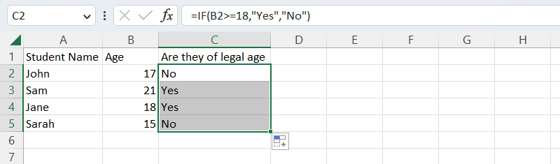
=IF(B2>=18,”Yes”,”No”)
This tells Excel that if the value of cell B2 is greater than or equal to 18, it should enter “Yes” in the target cell. If the value of cell B2 is less than 18, it should enter “No.”
The IF function in action.
Shimon Brathwaite / Foundry
Tip: When using functions like this, rather than entering the function repeatedly for each row, you can simply click and drag the tiny square on the bottom right of the cell that contains the function. Doing so will autofill each of the rows with the formula, and Excel will change your cell references to match. For example, when the formula we used in cell C2 that references cell B2 is autofilled into cell C3, it changes to reference cell B3 automatically.
Autofilling a formula to subsequent rows in the column.
Shimon Brathwaite / Foundry
Find more details at Microsoft’s IF function support page.
3. The SUMIF and COUNTIF functions
SUMIF is a more advanced SUM function that allows you to add up only the values in a range that meet the criteria you specify. To use this function, you must specify the range of cells to apply the criteria to, the criteria for inclusion, and, optionally, the sum range, which is the range of cells to total if that’s different from the initial range. The syntax is as follows:
=SUMIF(range,criteria,[sum_range])
Note that any criteria with text or mathematical or logical symbols must be enclosed in double quotes.
In the sales spreadsheet shown below, for example, suppose you want to total up only the sales that are more than $100. The criteria range is C2 to C9, and the criteria is “greater than 100.” Since you’re adding up the values in that same cell range (C2 to C9), you don’t need to supply a separate sum range. So your formula is:
=SUMIF(C2:C9,”>100″)
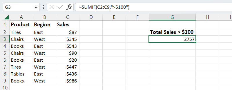
Using the SUMIF function.
Shimon Brathwaite / Foundry
What if instead you want to find the total for all sales in the East region only? To do that you’ll have to specify both the criteria range (cells B2 to B9) and the sum range (cells C2 to C9). This is the formula:
=SUMIF(B2:B9,B2,C2:C9)
Note that you don’t have to type out “East” for the criteria. You can simply type B2 or click the cell B2 to have Excel search for the text it contains.
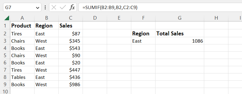
Using SUMIF with both a criteria range and a sum range.
Shimon Brathwaite / Foundry
There is a similar function called COUNTIF that lets you create a count of values that meet specified criteria. The syntax is as follows:
=COUNTIF(range,criteria)
So to count the total number of sales in the West region, for instance, you supply the range of cells to apply the criteria to (B2 to B9), followed by the criteria (“West” or cell B3). The formula is:
=COUNTIF(B2:B9,B3)
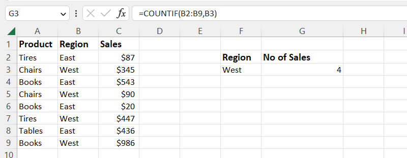
The COUNTIF function can instantly count up items that meet your criteria.
Shimon Brathwaite / Foundry
What if you want to apply multiple criteria to your data, such as calculating total sales for books in the East region, or counting the number of sales over $100 in the West region? Excel can do that too, via functions called SUMIFS and COUNTIFS. These functions use more complex syntax than SUMIF and COUNTIF. For more details, use cases, and best practices for all four of these functions, see Microsoft’s SUMIF, SUMIFS, COUNTIF, and COUNTIFS support pages.
4. The CONCAT function
This function is useful for piecing together text from different cells into one complete string. For instance, maybe you have a worksheet with different columns for people’s first and last names, but you want to put first and last names together. Other common use cases are completing an address, reference number, file path, or URL. The syntax is as follows:
=CONCAT(text1,text2,text3,…)
In this example we will use CONCAT to combine a list of first names and last names into a full name with a space in between. To do so we simply place the cursor in cell C2, type =CON and select CONCAT from the list of options that appears. Next, select the cell that contains the first name (A2) and add a comma, a blank space surrounded by quotation marks, and another comma. Then add the last name by selecting the adjacent cell (B2) and hit Enter. Here’s the full formula:
=CONCAT(A2,” “,B2)
Next, click and drag the bottom right of cell C2 to autofill the formula in all the other rows.
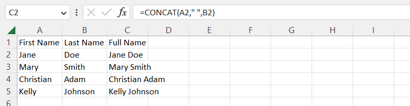
The CONCAT function combined the values from column A with those from column B.
Shimon Brathwaite / Foundry
For more details and examples, see Microsoft’s CONCAT function support page.
5. The VLOOKUP function
This is one of the most commonly used functions in Excel and a valuable data analysis tool. VLOOKUP lets you look up a value in a table and return information from other columns related to that value. It’s very useful for combining data from different lists or comparing two lists to find matching items. To use this function, you need to provide three to four pieces of information:
- The value you want to look for. This is known as the lookup value.
- The range of cells to look in. This is known as the table array.
- The column that contains the information you want to return, called the column index number.
- Optionally, the type of lookup you want to perform: TRUE or FALSE. This is known as the range lookup. FALSE means you want an exact match for the lookup value, while picking TRUE returns the best approximate match. If you don’t specify a range lookup, VLOOKUP defaults to TRUE.
The syntax is as follows:
=VLOOKUP(lookup_value,table_array,column_index_number,[range_lookup])
The lookup value must be in the first column of cells you specify in the table array. The leftmost column in the table array has a column index number of 1, with subsequent columns numbered 2, 3, and so on.
In this example, we’ll look up what region our employees work in. To do so, we first need to specify the value that we are going to search for: the employee name Mike (cell A2). Next, we need to highlight the entire cell range (table array) that we want to look in: cells F2:G8.
Then we specify which column holds the information that we want. Rather than picking the column itself, we count from left to right within the table array. Since the column that contains the region is the second from the left, type in 2.
Lastly, we enter the TRUE (best approximate match) or FALSE (exact match) option. TRUE is typically only used with numbers or when you aren’t sure if the value you want is in the table. Since we know the value we want is in the table, we will pick FALSE. Generally, FALSE is the better option, as it returns more accurate results.
This is the full formula:
=VLOOKUP(A2,F2:G8,2,FALSE)
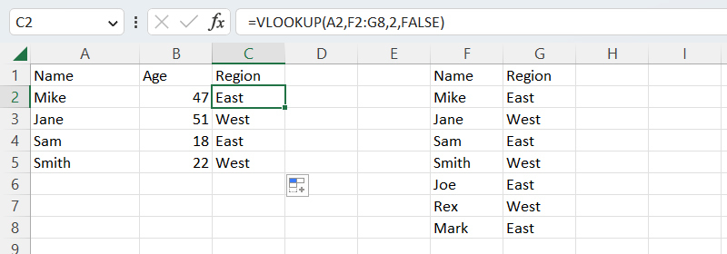
Use VLOOKUP to find values linked to other values in large data sets.
Shimon Brathwaite / Foundry
This is an oversimplified example using a small data set, but when you need to search through a spreadsheet with thousands (or tens of thousands) of cells, VLOOKUP is a huge time-saver and reduces the possibility of errors. For more details and examples, see Microsoft’s VLOOKUP function support page.
Using Copilot to create Excel formulas
Remembering all these different formulas and functions can be difficult, so another good approach for those who have access to Copilot in Excel (see details at the top of this story) is to use the AI tool to dynamically create formulas that meet your needs. Using Copilot, you can describe what you want the formula to do and have the AI generate the syntax for you. In this section we’ll demonstrate with two sample data sets.
To access Copilot, click the Copilot icon on your ribbon toolbar or at the bottom right of your screen.
To invoke Copilot, click its icon, which you might find in the ribbon toolbar up top or floating at the bottom right of your Excel window.
Shimon Brathwaite / Foundry
The Copilot sidebar opens along the right side of your spreadsheet. Type in a prompt describing the formula you want created — in this example, a simple formula that adds up all the sales values in the data set. Be sure to instruct Copilot where to place the formula:
Create a formula in B7 that sums all of the sales
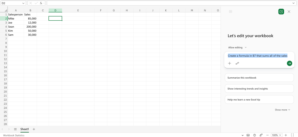
Describe the formula you want Copilot to create.
Shimon Brathwaite / Foundry
Click the submit arrow in the chat window, and Copilot will create and insert the formula to give you the result you want.
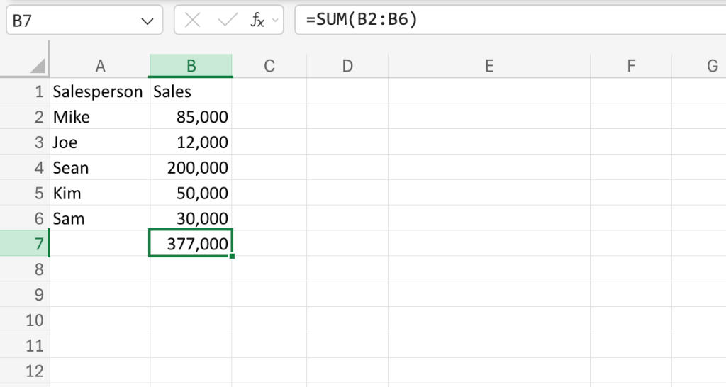
Copilot has inserted the correct Excel formula for the sum operation, with the result appearing in cell B7.
Shimon Brathwaite / Foundry
That was a simple one. Now try a more advanced example working from a more complex data set, as shown in the screenshot below.
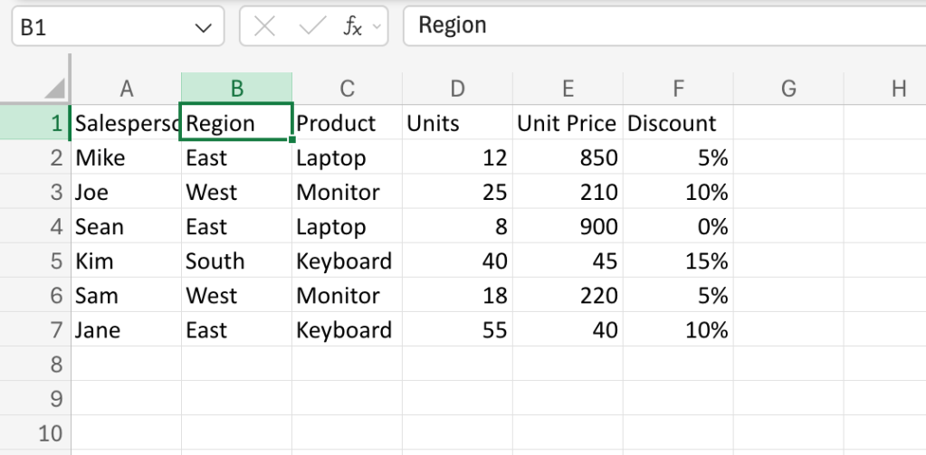
A more complex data set for our second example.
Shimon Brathwaite / Foundry
Try the following prompt:
Create a formula in G2 that calculates total revenue per unit while accounting for the discount on each purchase. Then fill the formula down for all rows and create a summary table showing total revenue by Region.
Click the submit arrow, and it should create something like this:
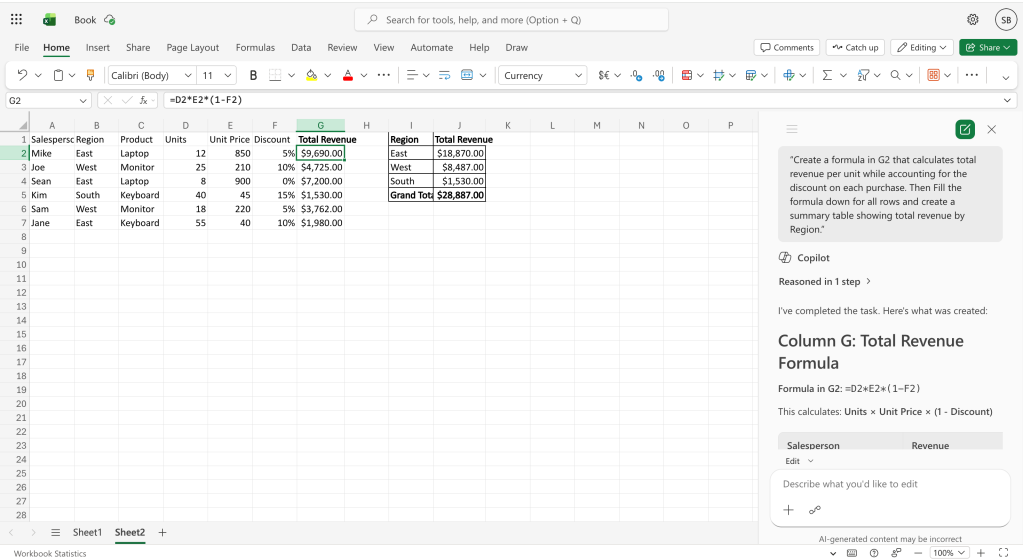
Copilot creates the requested formula and fills in the results.
Shimon Brathwaite / Foundry
(There’s a lot more you can have Copilot can do in Excel besides creating formulas. See our story “11 cool things Copilot can do in Excel.”)
Tip: It’s not required, but it can be helpful to format your spreadsheet as a table when working with Copilot. This helps define more clearly the exact cells for Copilot to use when it creates formulas or takes other actions on your data.
You’re just getting started
In this story you’ve seen how powerful formulas and functions can be in Excel — and we’ve only the scratched the surface of what they can do. Once you get comfortable using them, you can explore some of the myriad prebuilt functions Excel offers and learn how to build more complex formulas (including nesting functions). That’s all beyond the scope of this article, but a great place to start is Microsoft’s “Overview of formulas in Excel” support page, which includes links to several helpful tutorials.
For those who have access to it in Excel, experimenting with Copilot is another great way to learn. You can review the steps it took and the formulas it created to get a better understanding of how formulas work and what they’re capable of.
This story was originally published in May 2023 and updated in June 2026.
More Excel tips and how-tos:
Read the full article here